Hi,I’m trying to draw a 2D TDS spectrum of tungsten containing one trap.
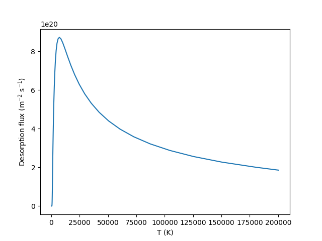
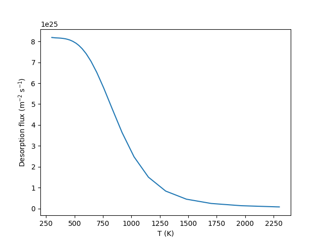
But I found the total flux need very long time to reach the peak and it won’t reduce to zero while the flux out of the trap drop to 0 very quickly.
And here’s my code:
import festim as F
model_2d = F.Simulation()
import numpy as np


wu = F.Material(
    id=1,
    D_0=1.93e-7,
    E_D=0.2,
    )
model_2d.materials = wu


from fenics import UnitSquareMesh, CompiledSubDomain, MeshFunction, plot

# creating a mesh with FEniCS
nx = ny = 20
mesh_fenics = UnitSquareMesh(nx, ny)

# marking physical groups (volumes and surfaces)
volume_markers = MeshFunction(
    "size_t", mesh_fenics, mesh_fenics.topology().dim())
volume_markers.set_all(1)

left_surface = CompiledSubDomain(
    'on_boundary && near(x[0], 0, tol)', tol=1e-14)
right_surface = CompiledSubDomain(
    'on_boundary && near(x[0], 1, tol)', tol=1e-14)
bottom_surface = CompiledSubDomain(
    'on_boundary && near(x[1], 0, tol)', tol=1e-14)
top_surface = CompiledSubDomain(
    'on_boundary && near(x[1], 1, tol)', tol=1e-14)

surface_markers = MeshFunction(
    "size_t", mesh_fenics, mesh_fenics.topology().dim() - 1)
surface_markers.set_all(0)

left_id = 1
top_id = 2
right_id = 3
bottom_id = 4
left_surface.mark(surface_markers, left_id)
right_surface.mark(surface_markers, right_id)
top_surface.mark(surface_markers, top_id)
bottom_surface.mark(surface_markers, bottom_id)


# creating mesh with festim
model_2d.mesh = F.Mesh(
    mesh=mesh_fenics,
    volume_markers=volume_markers,
    surface_markers=surface_markers
)

w_atom_density = 6.3e28  # atom/m3

trap_1 = F.Trap(
    k_0= 1.93e-7/ (1.1e-10**2 * 6 * w_atom_density),
    E_k=0.2,
    p_0=1e13,
    E_p=0.87,
    density=1.3e-3*w_atom_density,
    materials=wu,
    )

model_2d.traps = [trap_1]

model_2d.initial_conditions = [
	F.InitialCondition(field="1", value=1.3e-3*w_atom_density),
	F.InitialCondition(field="solute",value=0),
]

model_2d.boundary_conditions = [
        F.DirichletBC(surfaces=1, value=0, field=0),
	F.DirichletBC(surfaces=2, value=0, field=0),
        F.DirichletBC(surfaces=3, value=0, field=0),
	F.DirichletBC(surfaces=4, value=0, field=0),
]

ramp = 2  # K/s
model_2d.T = 300 + ramp * (F.t)

model_2d.dt = F.Stepsize(
    initial_value=0.01,
    stepsize_change_ratio=1.2,
    dt_min=1e-6,
)
model_2d.settings = F.Settings(
    absolute_tolerance=1e10,
    relative_tolerance=1e-10,
    final_time=1000,
    maximum_iterations=100,
)

derived_quantities =F.DerivedQuantities(
    [
	F.TotalVolume("solute", volume=1),
        F.TotalVolume("retention", volume=1),
        F.TotalVolume("1", volume=1),
        F.HydrogenFlux(surface=1),
        F.HydrogenFlux(surface=2),
	F.HydrogenFlux(surface=3),
	F.HydrogenFlux(surface=4),
	F.AverageVolume(field="T",volume=1),
    ]
)


model_2d.exports = [derived_quantities]
model_2d.initialise()
model_2d.run()

T = derived_quantities.filter(fields = "T").data
flux_left = derived_quantities.filter(fields="solute", surfaces=1).data
flux_top = derived_quantities.filter(fields="solute", surfaces=2).data
flux_right = derived_quantities.filter(fields="solute", surfaces=3).data
flux_buttom = derived_quantities.filter(fields="solute", surfaces=4).data
flux_trap1 = derived_quantities.filter(fields="1").data
mobile = derived_quantities.filter(fields="solute", instances=F.TotalVolume).data
total = derived_quantities.filter(fields="retention").data

flux_total = -np.array(flux_left) - np.array(flux_top) - np.array(flux_right) - np.array(flux_buttom)
import matplotlib.pyplot as plt
#plt.plot(T, mobile, linewidth=3)
plt.plot(T, flux_total)
#plt.plot(T,flux_trap1)
plt.ylabel(r"Desorption flux (m$^{-2}$ s$^{-1}$)")
plt.xlabel(r"T (K)")
plt.savefig('2d.png')
This really confused me,I’m looking forward to your reply.
Thank you!