Hello, I am using FESTIM to understand hydrogen retention in displacement damage created by neutron radiation.
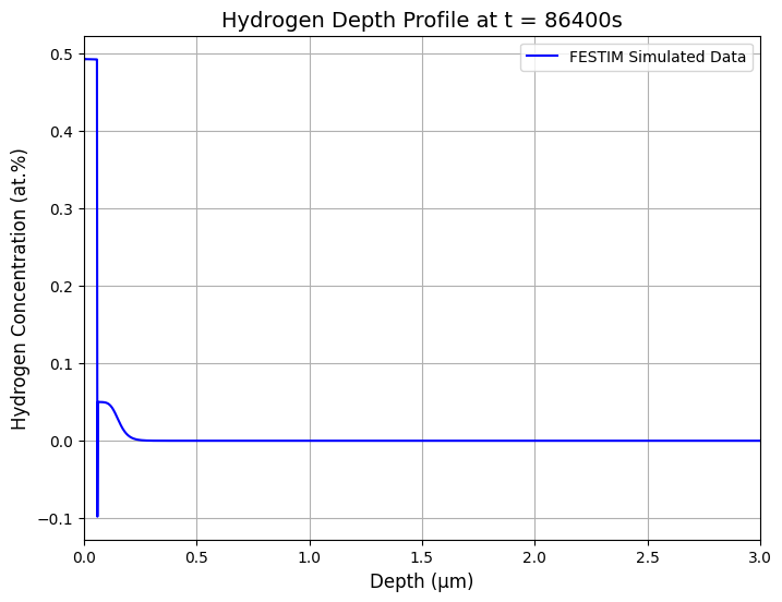
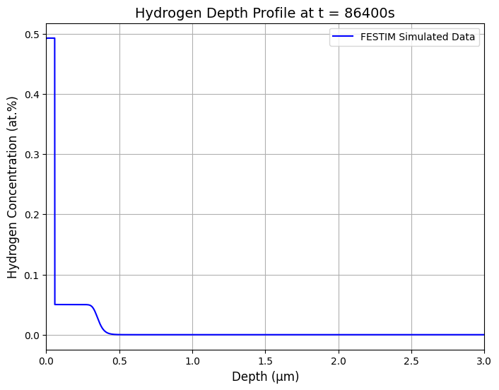
I wanted to know if I don’t put Drichlet boundary conditions, can I still get depth profiles of deuterium in depth, only using TDS. Also, I don’t see an example to plot depth profiles.
Any help would be appreciated
Heres my code,
import festim as F
import sympy as sp
import numpy as np
import matplotlib.pyplot as plt
import pandas as pd
from scipy.interpolate import make_interp_spline
Load the Excel file and experimental data
file_path = ‘seq 370K.xlsx’ # Replace with your file path
sheet_data = pd.read_excel(file_path, sheet_name=‘Sheet2’) # Experimental 370K data
x = sheet_data[‘Temp(K)’] # Experimental temperature
y = sheet_data[‘D/m2Ss’] # Experimental flux
Function to run FESTIM simulation
def run_festim_simulation():
# Initialize the simulation
model = F.Simulation()
model.log_level = 40
# Define the mesh
L = 1e-3 # Full thickness, 1 mm in meters
vertices = np.concatenate(
[
np.linspace(0, 1e-8, num=200), # High resolution near the surface
np.linspace(1e-8, 4e-6, num=200), # Moderate resolution for shallow implantation
np.linspace(4e-6, L, num=100), # Reduced resolution in the bulk region (ends at L)
np.linspace(L, L + 1e-8, num=200), # High resolution near the far end (extends slightly beyond L)
]
)
model.mesh = F.MeshFromVertices(vertices)
# Define material properties
eurofer = F.Material(id=1, D_0=1.5e-7, E_D=0.15)
model.materials = eurofer
# Define atomic density and lattice parameters
eurofer_density = 8.59e28 # atoms/m3
lambda_lat = eurofer_density ** (-1 / 3)
nu_dt=4e13
D0 = 1.5e-7
nu_bs = D0/ lambda_lat**2
incident_flux = 1.62e17 # D atoms/m2s
nu_tr=D0/lambda_lat**2
n_IS = 6 * eurofer_density
# Define the source term
implantation_time = 24 * 3600 # 24 hours in seconds
# distr = sp.Piecewise((1, F.x < 5.33e-6), (0, True))
implanted_flux = incident_flux * 0.4
ion_flux = sp.Piecewise((implanted_flux, F.t <= implantation_time), (0, True))
source_term = F.ImplantationFlux(
flux=ion_flux, imp_depth=-2.4e-9, width=1.2e-9/np.sqrt(2), volume=1
)
model.sources = [source_term]
# Define traps
distrr = 1 / (1 + sp.exp((F.x - 2.0e-6) / 0.9e-6))
# trap_1 = F.Trap(
# # k_0=eurofer.D_0 * 6 * eurofer_density/(lambda_lat**2),
# k_0=nu_tr/n_IS,
# E_k=0.15,
# p_0=nu_dt,
# E_p=1.42,
# density=1e-5 * eurofer_density,
# materials=eurofer,
# )
trap_1 = F.Trap(
# k_0=eurofer.D_0 * 6 * eurofer_density/(lambda_lat**2),
k_0=nu_tr/n_IS,
E_k=0.15, #E_trap=E_diff
p_0=nu_dt, #de-trap attempt frequency
E_p=1.45,
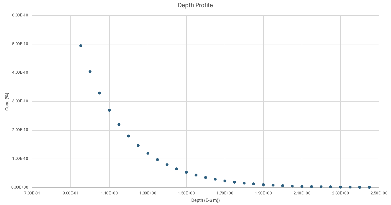
density = sp.Piecewise(
(0.00493 * eurofer_density, F.x < 0.05894e-6), # High concentration near the surface
(5.01299e-4 * eurofer_density, F.x < 1.32615e-6), # Medium concentration at intermediate depth
(9.39544e-5 * eurofer_density, F.x < 1.94502e-6), # Lower concentration further in depth
(1.97561e-5 * eurofer_density, F.x < 5.3046e-6), # Very low concentration deeper
(0, True) # No concentration beyond the maximum depth
),
    materials=eurofer,
)
model.traps = [trap_1]

# Define boundary conditions
model.boundary_conditions = [F.DirichletBC(surfaces=[1, 2], value=0, field=0)]

# Define temperature profile with ramp
tds_temp_start = 290  # Initial TDS temperature after implantation, in Kelvin
final_temperature =650 # Final temperature in Kelvin
ramp_rate = 0.05  # Temperature ramp rate, K/s
start_tds = implantation_time + 20  # Time when the ramp starts

# Calculate the duration of the ramp
ramp_duration = (final_temperature - tds_temp_start) / ramp_rate
end_tds = start_tds + ramp_duration  # Time when the ramp ends
t_load=370 #K
model.T = F.Temperature(
    value=sp.Piecewise(
        (tds_temp_start, F.t <= start_tds),  # Constant temperature before ramp starts
        (tds_temp_start + ramp_rate * (F.t - start_tds), F.t <= end_tds),  # Ramp
        (final_temperature, True),  # Constant final temperature after the ramp
    )
)


model.dt = F.Stepsize(
initial_value=1e-5,
stepsize_change_ratio=1.25,
max_stepsize=500,
dt_min=1e-5,
milestones=[implantation_time, start_tds, end_tds],
)
model.settings = F.Settings(
absolute_tolerance=1e7,
relative_tolerance=1e-13,
final_time=end_tds,
traps_element_type=“DG”,
)
# Define derived quantities
list_of_derived_quantities = F.DerivedQuantities(
[
    # F.TotalVolume("solute", volume=1),
    F.TotalVolume("retention", volume=1),
    F.TotalVolume("1", volume=1),
    # F.TotalVolume("2", volume=1),
    F.AverageVolume("T", volume=1),
    F.HydrogenFlux(surface=1),
    F.HydrogenFlux(surface=2),
    # F.AdsorbedHydrogen(surface=1),
    # F.AdsorbedHydrogen(surface=2),
], show_units=True,
 filename="./my_derived_quantities.csv",
)
model.exports = [list_of_derived_quantities]
# Run the simulation
model.initialise()
model.run()
print("Simulation completed. Checking exports...")

# Post-process results
t = list_of_derived_quantities.t
flux_left = list_of_derived_quantities.filter(fields="solute", surfaces=1).data
flux_right = list_of_derived_quantities.filter(fields="solute", surfaces=2).data
flux_total = -np.array(flux_left) - np.array(flux_right)

trap_1 = list_of_derived_quantities.filter(fields="1").data
# trap_dpa = derived_quantities.filter(fields="2").data
T = list_of_derived_quantities.filter(fields="T").data

   # Extract data after the TDS start
indexes = np.where(np.array(t) > start_tds)
t = np.array(t)[indexes]
T = np.array(T)[indexes]
flux_total = np.array(flux_total)[indexes]

# Remove duplicates from T and flux_total
T, unique_indices = np.unique(T, return_index=True)
flux_total = flux_total[unique_indices]

# Smooth FESTIM data
T_smooth = np.linspace(T.min(), T.max(), 700)
flux_total_smooth = make_interp_spline(T, flux_total)(T_smooth)

# Normalize the flux
flux_total_smooth_normalized = flux_total_smooth / np.max(flux_total_smooth)

return T_smooth, flux_total_smooth_normalized
Call the simulation and retrieve the results
T_smooth, flux_total_smooth_normalized = run_festim_simulation()
Initialize the plot
fig, ax1 = plt.subplots(figsize=(10, 6))
Plot experimental data
exp_370_plot, = ax1.plot(
x, y / np.max(y), linestyle=“dashed”, label=“Exp 370K”, marker=“o”, color=“tab:blue”
)
Plot simulation data
ax1.plot(
T_smooth,
flux_total_smooth_normalized,
linestyle=“solid”,
color=“tab:red”,
label=“FESTIM 370K”,
)
Customize plot
ax1.set_xlabel(“Temperature (K)”, fontsize=12)
ax1.set_ylabel(r"Desorption flux (m$^{-2} s^{-1}$)", fontsize=12, color=“tab:blue”)
ax1.tick_params(axis=“y”, labelcolor=“tab:blue”)
ax1.set_xlim(300, 800)
ax1.legend(loc=“upper left”)
ax1.grid(alpha=0.3)
plt.title(“Comparison of FESTIM and Experimental Desorption Flux”)
plt.tight_layout()
plt.show()