Hi !Hope you’re having a good day! ![]() I’m trying to use FESTIM to get the time-dependent hydrogen concentration at 1, 5, and 10 microns near the surface during the injection process—it’s one of the final bits of my project, and honestly, my boss is really on my case to wrap this up.
I’m trying to use FESTIM to get the time-dependent hydrogen concentration at 1, 5, and 10 microns near the surface during the injection process—it’s one of the final bits of my project, and honestly, my boss is really on my case to wrap this up.
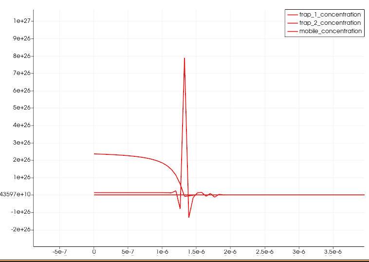
Earlier, I tried coarsening the mesh near the surface, and while the code ran without errors, it just spat out all zeros (bummer!). Now, I’m attempting a finer mesh, but the residuals keep creeping up over time, which eventually resulted in time step reaching the minimum value.
Quick heads-up: Some parts of this were AI-generated, so it might come across as a bit wordy or over-explained—I apologize for that! If you’ve got any tips or could point me , I’d be so grateful. Thanks a ton for your time and help! ![]()
My code :
import festim as F
my_model = F.Simulation()
my_model.log_level = 20
import numpy as np
import sympy as sp
import os

output_dir = "output"
if not os.path.exists(output_dir):
   os.makedirs(output_dir)
   print(f"Output directory created: {output_dir}")

# Mesh generation with refined regions near the surface

surface_region_1 = np.linspace(0, 10e-9, num=200)

surface_region_2 = np.linspace(10e-9, 50e-9, num=160)

surface_region_3 = np.linspace(50e-9, 200e-9, num=150)

surface_region_4 = np.linspace(200e-9, 1e-6, num=320)

mid_region_1 = np.linspace(1e-6, 10e-6, num=720)

mid_region_2 = np.linspace(10e-6, 100e-6, num=1800)

mid_region_3 = np.linspace(100e-6, 1e-3, num=1800)

far_region = np.linspace(1e-3, 3e-3, num=400)
vertices = np.concatenate([
   surface_region_1,
   surface_region_2,
   surface_region_3,
   surface_region_4,
   mid_region_1,
   mid_region_2,
   mid_region_3,
   far_region
])
my_model.mesh = F.MeshFromVertices(vertices)

# Tungsten material properties
tungsten = F.Material(
   id=1,
   D_0=2.9e-7,  # Pre-exponential factor for diffusion (m2/s)
   E_D=0.39,  # Activation energy for diffusion (eV)
)
my_model.materials = tungsten

# Total implantation time in seconds
implantation_time = 9000  # s

# Time-dependent ion flux profile for LTD experiment
# The flux changes at different time intervals to simulate experimental conditions
ion_flux = sp.Piecewise(
   (2.3e22 * F.t / 200, (F.t >= 0) & (F.t <= 200)),
   (2.3e22, (F.t > 200) & (F.t <= 1800)),
   (1.9e22, (F.t > 1800) & (F.t <= 3600)),
   (1.03e22, (F.t > 3600) & (F.t <= 5400)),
   (6.23e21, (F.t > 5400) & (F.t <= 7200)),
   (2.5e21, (F.t > 7200) & (F.t <= 9000)),
   (0, True)
)
iflux = sp.simplify(ion_flux)
print(iflux)

# Hydrogen implantation source term
# imp_depth: implantation depth (m)
# width: standard deviation of Gaussian implantation profile (m)
source_term = F.ImplantationFlux(
   flux=ion_flux,  # H/m2/s
   imp_depth=4e-9,  # m
   width=2e-9,  # m
   volume=1
)
my_model.sources = [source_term]

# Tungsten atomic density (atoms/m3)
w_atom_density = 6.3e28  # atom/m3

# Dislocation trap properties
dislocation_trap = F.Trap(
   k_0=2.9e12 / w_atom_density,  # Trap formation attempt frequency (s-1)
   E_k=0.29,  # Trap formation activation energy (eV)
   p_0=1e13,  # Detrap attempt frequency (s-1)
   E_p=1.1,  # Detrap activation energy (eV)
   density=4e-3 * w_atom_density,  # Trap density (m-3)
   materials=tungsten
)

# Vacancy trap properties
vacancy_trap = F.Trap(
   k_0=2.9e12 / w_atom_density,
   E_k=0.29,
   p_0=1e13,
   E_p=1.5,
   density=2e-4 * w_atom_density,
   materials=tungsten
)
my_model.traps = [dislocation_trap, vacancy_trap]

# Dirichlet boundary conditions (zero concentration at both surfaces)
my_model.boundary_conditions = [
   F.DirichletBC(surfaces=[1, 2], value=0, field=0)
]

# Time-dependent temperature profile for LTD experiment
# Simulates cooling steps during implantation
implantation_temp = sp.Piecewise(
   (570, F.t <= 1800),
   (570 - (570 - 520) / (1850 - 1800) * (F.t - 1800), (F.t > 1800) & (F.t <= 1850)),
   (520, (F.t > 1850) & (F.t <= 3600)),
   (520 - (520 - 470) / (3650 - 3600) * (F.t - 3600), (F.t > 3600) & (F.t <= 3650)),
   (470, (F.t > 3650) & (F.t <= 5400)),
   (470 - (470 - 420) / (5450 - 5400) * (F.t - 5400), (F.t > 5400) & (F.t <= 5450)),
   (420, (F.t > 5450) & (F.t <= 7200)),
   (420 - (420 - 370) / (7250 - 7200) * (F.t - 7200), (F.t > 7200) & (F.t <= 7250)),
   (370, (F.t > 7250) & (F.t <= 9000)),
   (300, True)
)
it = sp.simplify(implantation_temp)
print(it)

# TDS heating rate (K/s)
temperature_ramp = 1  # K/s
# Start time for TDS phase (after implantation)
start_tds = implantation_time + 50  # s

# Create dense time points list for milestones - especially around critical points
temp_change_points = [1800, 1850, 3600, 3650, 5400, 5450, 7200, 7250, 9000, 200]
time_points = list(range(0, 5, 1))  # First 5 seconds
time_points += list(range(5, 20, 2))  # 5-20 seconds
time_points += list(range(20, 100, 5))  # 20-100 seconds
time_points += list(range(100, 1000, 50))  # 100-1000 seconds
time_points += list(range(1000, implantation_time + 1, 200))  # 1000-9000 seconds
time_points += [implantation_time, start_tds]
for point in temp_change_points:
   time_points.extend([point - 10, point - 5, point, point + 5, point + 10])

# Temperature profile definition
# Implantation phase: time-dependent temperature
# Waiting phase: constant 300K
# TDS phase: linear heating at 1K/s
my_model.T = sp.Piecewise(
   (implantation_temp, F.t < 9000),
   (300, (F.t > 9000) & (F.t < start_tds)),
   (300 + temperature_ramp * (F.t - start_tds), True)
)

# Adaptive time stepping strategy
# Smaller steps at critical time points for numerical stability
my_model.dt = F.Stepsize(
   initial_value=0.01,
   stepsize_change_ratio=1,
   max_stepsize=lambda t: 0.001 if t < 10 else (0.01 if t < 100 else (0.1 if t < 1000 else 1)),
   dt_min=1e-10,
   milestones=sorted(set(time_points)),
)

# Simulation settings
my_model.settings = F.Settings(
   absolute_tolerance=1e22,
   relative_tolerance=1e-5,
   final_time=15000,
)

# Define derived quantities to export
list_of_derived_quantities = [
   F.TotalVolume("solute", volume=1),
   F.TotalVolume("retention", volume=1),
   F.TotalVolume("1", volume=1),  # Dislocation traps
   F.TotalVolume("2", volume=1),  # Vacancy traps
   F.HydrogenFlux(surface=1),
   F.HydrogenFlux(surface=2)
]

# Add point monitoring at specific locations (5um, 10um, 1um)
point_5um_trap1 = F.PointValue(field="1", x=5e-6)  # Dislocation traps
point_5um_trap2 = F.PointValue(field="2", x=5e-6)  # Vacancy traps
point_10um_trap1 = F.PointValue(field="1", x=10e-6)
point_10um_trap2 = F.PointValue(field="2", x=10e-6)
point_1um_trap1 = F.PointValue(field="1", x=1e-6)  # 1 micron
point_1um_trap2 = F.PointValue(field="2", x=1e-6)

# Add point monitoring to export list
list_of_derived_quantities.append(point_5um_trap1)
list_of_derived_quantities.append(point_5um_trap2)
list_of_derived_quantities.append(point_10um_trap1)
list_of_derived_quantities.append(point_10um_trap2)
list_of_derived_quantities.append(point_1um_trap1)
list_of_derived_quantities.append(point_1um_trap2)

# Create exporter for derived quantities
derived_quantities = F.DerivedQuantities(
   list_of_derived_quantities,
   filename=os.path.join(output_dir, "LTD-temp-data.csv"),
   show_units=True,
)
my_model.exports = [derived_quantities]

# Initialize and run the simulation
my_model.initialise()
my_model.run()

# Post-processing: extract and save required data
import pandas as pd

# Read all data
temp_data_path = os.path.join(output_dir, "LTD-temp-data.csv")
df = pd.read_csv(temp_data_path)

# Extract data at 5um, 10um, and 1um
point_columns = [col for col in df.columns if "PointValue" in col]

if len(point_columns) >= 6:
   # Total trapped hydrogen concentration at 5um
   df_5um = df[['t (s)', point_columns[0], point_columns[1]]].copy()
   df_5um['Total trapped'] = df_5um[point_columns[0]] + df_5um[point_columns[1]]
   df_5um = df_5um[['t (s)', 'Total trapped']]
   df_5um.columns = ['Time (s)', 'Concentration (m^-3)']

   # Total trapped hydrogen concentration at 10um
   df_10um = df[['t (s)', point_columns[2], point_columns[3]]].copy()
   df_10um['Total trapped'] = df_10um[point_columns[2]] + df_10um[point_columns[3]]
   df_10um = df_10um[['t (s)', 'Total trapped']]
   df_10um.columns = ['Time (s)', 'Concentration (m^-3)']

   # Total trapped hydrogen concentration at 1um
   df_1um = df[['t (s)', point_columns[4], point_columns[5]]].copy()
   df_1um['Total trapped'] = df_1um[point_columns[4]] + df_1um[point_columns[5]]
   df_1um = df_1um[['t (s)', 'Total trapped']]
   df_1um.columns = ['Time (s)', 'Concentration (m^-3)']

   # Keep only implantation phase data (t <= implantation_time) with 500s interval
   df_5um = df_5um[df_5um['Time (s)'] <= implantation_time]
   df_5um = df_5um[df_5um['Time (s)'] % 500 == 0]
   df_10um = df_10um[df_10um['Time (s)'] <= implantation_time]
   df_10um = df_10um[df_10um['Time (s)'] % 500 == 0]
   df_1um = df_1um[df_1um['Time (s)'] <= implantation_time]
   df_1um = df_1um[df_1um['Time (s)'] % 500 == 0]

   # Save data to CSV files
   df_5um.to_csv(os.path.join(output_dir, "LTD-5um.csv"), index=False)
   df_10um.to_csv(os.path.join(output_dir, "LTD-10um.csv"), index=False)
   df_1um.to_csv(os.path.join(output_dir, "LTD-1um.csv"), index=False)
   print(f"Successfully saved 5um, 10um and 1um data to {output_dir} directory")
else:
   print("Warning: Not enough PointValue columns found to extract data")

# Generate TDS curve (desorption phase only)
t = df['t (s)'].values
flux_left = df[[col for col in df.columns if "surface 1" in col and "solute" in col]].values.flatten()
flux_right = df[[col for col in df.columns if "surface 2" in col and "solute" in col]].values.flatten()
flux_total = -flux_left - flux_right

# Only take desorption phase data (t >= implantation_time)
t_desorption = t[t >= implantation_time]
flux_total_desorption = flux_total[t >= implantation_time]

import matplotlib.pyplot as plt
plt.figure(figsize=(10, 6))
plt.plot(t_desorption, flux_total_desorption, linewidth=3)
plt.ylabel(r"Desorption flux (m$^{-2}$ s$^{-1}$)")
plt.xlabel(r"Time (s)")
plt.title("TDS Curve")
plt.grid(True)
tds_path = os.path.join(output_dir, 'LTD-tds.png')
plt.savefig(tds_path)
plt.close()
print(f"TDS curve successfully saved to {tds_path}")