Hi everyone,
I’m doing a simple series of permeation experiments with a set of different values for each parameter (diffusivity, Temperature and such), specifically, a full factorial DOE. I’m having trouble with the simulation stopping without an error message when I increase the time or just when running the script, such as with the case that I am presenting.
The script is based on task 3, with a little modification to make it suitable for the full DOE. I don’t have much background with Finite Element Analysis or solvers, but I believe the issue might be there. Hope someone can point me in the right direction. I’ll paste the code below.
import festim as F
import numpy as np
Temp=298 #K
Pres=1 #bar
d_0=1e-9 #m2/s
e_D=5 #KJ/mol
s_0=10 #mol/m3*MPa^0.5
e_S=5 #KJ/mol
Thick=0.1 #mm
Presc=Pres*1e5 #Pa
e_Dc=e_D*0.010364 #eV
s_0c=s_0*6.022e23 #H/m3*0.5Pa
e_Sc=e_S*0.010364 #eV
Thickc=0.1*1e-4
my_model = F.Simulation()
my_model.mesh = F.MeshFromVertices(
vertices=np.linspace(0, Thickc , num=1001)
)
my_model.materials = F.Material(
id=1,
D_0=d_0, #m2/s
E_D=e_Dc #eV
)
my_model.T = F.Temperature(
value=Temp
)
my_model.boundary_conditions = [
F.SievertsBC(
surfaces=1,
S_0=s_0c,
E_S=e_Sc,
pressure=Presc
),
F.DirichletBC(
surfaces=2,
value=0,
field=0
)
]
my_model.settings = F.Settings(
absolute_tolerance=1e-1,
relative_tolerance=1e-1,
final_time=500 # s
)
my_model.dt = F.Stepsize(
initial_value=1/20,
dt_min=1e-2
)
derived_quantities = F.DerivedQuantities([F.HydrogenFlux(surface=2)])
my_model.exports = [derived_quantities]
my_model.initialise()
my_model.run()
times = derived_quantities.t
computed_flux = derived_quantities.filter(surfaces=2).data
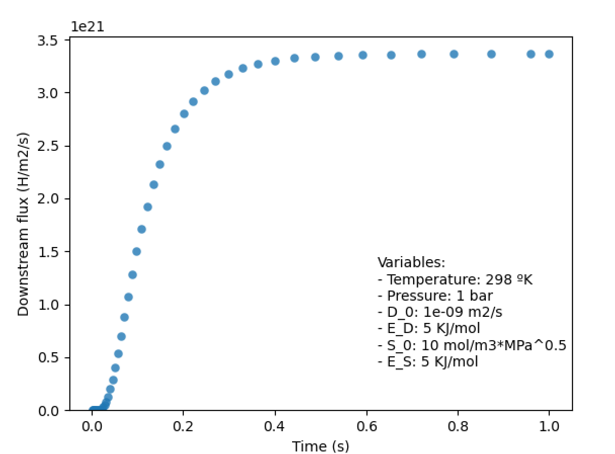
import matplotlib.pyplot as plt
plt.scatter(times, np.abs(computed_flux), alpha=0.1, label="computed",linewidths=0.1)
plt.ylim(bottom=0)
plt.xlabel("Time (s)")
plt.ylabel("Downstream flux (H/m2/s)")
# Add a footnote below and to the right side of the chart
plt.figtext(
0.6, 0.2,
f"Variables:\n- Temperature: {Temp} ºK\n- Pressure: {Pres} bar, {Presc} Pa\n- D_0: {d_0} m2/s \n- E_D: {e_D} KJ/mol, {e_Dc} eV\n- S_0: {s_0} mol/m3*MPa^0.5, {s_0c} H/m3*Pa^0.5\n- E_S: {e_S} KJ/mol, E_S: {e_Sc} eV",
ha="left",
fontsize=10,
)
plt.show()
Thanks to everyone for reading and let me know if I can give any more information. The error I get, if you call it that, is the following, the simulation just stops at a certain number, in this case 0.5%.