Inhomogeneous Dirichlet BC from csv file

ehodille · July 22, 2024, 9:57am

I have a y[m],cm[m-3] csv file and I would like to apply these values as an inhomogeneous Dirichlet boundary condition along one of the 1D boundary of my domain (here is a small sketch, if understandable).

I created a interpolation function with scipy.interpolate.interp1d called cm_f

  input_file_cm = 'concentration.csv'
  data = np.loadtxt(input_file_cm,skiprows=8)
  y = data[:,0]-data[0,0]
  cm = data[:,1]
  cm_f = interp1d(y,cm)

and I thought I could use that directly in the value argument of DirichletBC()

hydrogen_BFS = F.DirichletBC(
     value = bc.cm_f,
     surfaces = id.id_BFS,
     field=0
)

However, the execution of FESTIM reply during the “Defining boundary conditions phase”

I have been told that sympy.Piecewise could do the job too (but there are around 200 data points, is it ok ?).

thank you very much if someone has an idea

remidm · July 22, 2024, 10:48am

Hi @ehodille

A few tips for the future:

if you can post error messages as code blocks (using triple ``` ) this would help with things like googling error messages and such
the code blocks that you added are not reproducible (ie I can not just run them and reproduce your issue). For example, I don’t know what the variables bc and id are in bc.cm_f and id.id_BFS, respectively.
To get an answer quickly, it is recommended to produce what we call a MWE (Minimal Working Example).

In your case, I was able to reproduce what I believe is your issue with this MWE (although 1D):

import festim as F
import numpy as np

my_model = F.Simulation()

my_model.mesh = F.MeshFromVertices(vertices=np.linspace(0, 7e-6, num=1001))

my_model.materials = F.Material(id=1, D_0=1e-7, E_D=0.2)

my_model.T = F.Temperature(value=300)

from scipy.interpolate import interp1d

y = [0, 1, 2, 3]
cm = [0, 2, 3, 5]
cm_f = interp1d(y, cm)

my_model.boundary_conditions = [
    F.DirichletBC(surfaces=[1], value=cm_f, field=0),
]


my_model.settings = F.Settings(
    absolute_tolerance=1e-1, relative_tolerance=1e-10, transient=False  # s
)


my_model.initialise()

my_model.run()

and the error message is:

Defining initial values
Defining variational problem
Defining source terms
Defining boundary conditions
Traceback (most recent call last):
  File "/home/remidm/mikhail/test.py", line 28, in <module>
    my_model.initialise()
  File "/home/remidm/miniconda3/envs/festim-env-mikhail/lib/python3.11/site-packages/festim/generic_simulation.py", line 298, in initialise
    self.h_transport_problem.initialise(self.mesh, self.materials, self.dt)
  File "/home/remidm/miniconda3/envs/festim-env-mikhail/lib/python3.11/site-packages/festim/h_transport_problem.py", line 77, in initialise
    self.create_dirichlet_bcs(materials, mesh)
  File "/home/remidm/miniconda3/envs/festim-env-mikhail/lib/python3.11/site-packages/festim/h_transport_problem.py", line 219, in create_dirichlet_bcs
    bc.create_dirichletbc(
  File "/home/remidm/miniconda3/envs/festim-env-mikhail/lib/python3.11/site-packages/festim/boundary_conditions/dirichlets/dirichlet_bc.py", line 79, in create_dirichletbc
    self.create_expression(T)
  File "/home/remidm/miniconda3/envs/festim-env-mikhail/lib/python3.11/site-packages/festim/boundary_conditions/dirichlets/dirichlet_bc.py", line 29, in create_expression
    value_BC = sp.printing.ccode(self.value)
               ^^^^^^^^^^^^^^^^^^^^^^^^^^^^^
  File "/home/remidm/miniconda3/envs/festim-env-mikhail/lib/python3.11/site-packages/sympy/printing/codeprinter.py", line 752, in ccode
    return c_code_printers[standard.lower()](settings).doprint(expr, assign_to)
           ^^^^^^^^^^^^^^^^^^^^^^^^^^^^^^^^^^^^^^^^^^^^^^^^^^^^^^^^^^^^^^^^^^^^
  File "/home/remidm/miniconda3/envs/festim-env-mikhail/lib/python3.11/site-packages/sympy/printing/codeprinter.py", line 162, in doprint
    expr = _handle_assign_to(expr, assign_to)
           ^^^^^^^^^^^^^^^^^^^^^^^^^^^^^^^^^^
  File "/home/remidm/miniconda3/envs/festim-env-mikhail/lib/python3.11/site-packages/sympy/printing/codeprinter.py", line 146, in _handle_assign_to
    return sympify(expr)
           ^^^^^^^^^^^^^
  File "/home/remidm/miniconda3/envs/festim-env-mikhail/lib/python3.11/site-packages/sympy/core/sympify.py", line 465, in sympify
    raise SympifyError('cannot sympify object of type %r' % type(a))
sympy.core.sympify.SympifyError: SympifyError: "cannot sympify object of type <class 'scipy.interpolate._interpolate.interp1d'>"

Although in your case you seem to have a SyntaxError as well

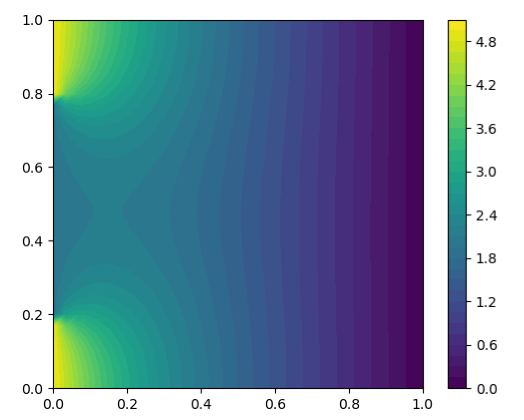
Yes you could use sympy.Piecewise. Consider the following example where we have a unit square, the data-based BC on the left and c=0 on the right:

import festim as F
import fenics as f


# make 2D unit square mesh and mark cells and facets
# left boundary is tagged with id 1 and right boundary with id 2
nx = ny = 30
fenics_mesh = f.UnitSquareMesh(nx, ny)


volume_markers = f.MeshFunction("size_t", fenics_mesh, fenics_mesh.topology().dim())
volume_markers.set_all(1)

surface_markers = f.MeshFunction(
    "size_t", fenics_mesh, fenics_mesh.topology().dim() - 1
)
surface_markers.set_all(0)


class Left(f.SubDomain):
    def inside(self, x, on_boundary):
        return on_boundary and f.near(x[0], 0.0)


class Right(f.SubDomain):
    def inside(self, x, on_boundary):
        return on_boundary and f.near(x[0], 1.0)


left = Left()
left.mark(surface_markers, 1)
right = Right()
right.mark(surface_markers, 2)

# FESTIM MODEL

my_model = F.Simulation()

my_model.mesh = F.Mesh(
    fenics_mesh, volume_markers=volume_markers, surface_markers=surface_markers
)
my_model.materials = F.Material(id=1, D_0=1e-7, E_D=0.2)

my_model.T = F.Temperature(value=300)

import sympy as sp

cm_f = sp.Piecewise(
    (5, F.y < 0.2), (2, F.y < 0.5), (3, F.y < 0.5), (2, F.y < 0.8), (5, True)
    # note instead of having a step function you can work how linear interpolation too
)


my_model.boundary_conditions = [
    F.DirichletBC(surfaces=[1], value=cm_f, field=0),
    F.DirichletBC(surfaces=[2], value=0, field=0),
]


my_model.settings = F.Settings(
    absolute_tolerance=1e-1, relative_tolerance=1e-10, transient=False  # s
)

my_model.initialise()

my_model.run()

CS = f.plot(my_model.h_transport_problem.u)
import matplotlib.pyplot as plt

plt.colorbar(CS)
plt.show()

Produces:

You could make this more generic by doing something like:

# your data
y = [0, 0.2, 0.5, 0.8, 1]
cm = [5, 2, 3, 2, 5]

list_of_tuples = [(cm_val, F.y < y) for cm_val, y in zip(cm, y[1:])]
list_of_tuples.append((cm[-1], True))

cm_f = sp.Piecewise(*list_of_tuples)

Now if I remember well, this kind of breaks (or at least is extremely long) when you have many more datapoints.

Instead, you could replace the BC in the previous code by:

class InterpolatedExpression(f.UserExpression):
    def __init__(self, f):
        super().__init__()
        self.f = f

    def eval(self, value, x):
        y = x[1]
        value[0] = self.f(y)

    def value_shape(self):
        # scalar value
        return ()


class DirichletBCFromData(F.DirichletBC):
    def __init__(self, surfaces, f, field):
        value = InterpolatedExpression(f)
        super().__init__(surfaces, value, field)

    # override the create_expression method
    def create_expression(self, T):
        self.expression = self.value


from scipy.interpolate import interp1d

# your data
y = [0, 0.2, 0.5, 0.8, 1]
cm = [5, 2, 3, 2, 5]
cm_f = interp1d(y, cm)

my_model.boundary_conditions = [
    DirichletBCFromData(surfaces=[1], f=cm_f, field=0),
    F.DirichletBC(surfaces=[2], value=0, field=0),
]

And this produces:

Here’s what we did:

Make our custom DirichletBC class because the one in FESTIM only allows value to be a float or a sympy.Expression. And override the create_expression method
Make a fenics.UserExpression class that gets a value from a interp1d object from the y-value.
make an instance of the custom DirichletBC and then give this to our FESTIM model

remidm · July 22, 2024, 10:53am

The second approach scales well as we increase the number of datapoints. For example, using 10000 points:

from scipy.interpolate import interp1d
import numpy as np

# your data
y = np.linspace(0, 1, num=10000)
cm = 1 + np.sin(2 * np.pi * y)
cm_f = interp1d(y, cm)

my_model.boundary_conditions = [
    DirichletBCFromData(surfaces=[1], f=cm_f, field=0),
    F.DirichletBC(surfaces=[2], value=0, field=0),
]

Produces:

and runs in less than a second on my laptop

ehodille · July 22, 2024, 1:22pm

Thank you very much, I used the 2nd method and it works perfectly without any time issue.

remidm · July 22, 2024, 1:38pm

We could potentially provide native support in FESTIM for this. You are welcome to open a PR!

remidm · July 23, 2024, 7:19am

@ehodille I also took the opportunity to adapt this example to a temperature field from a list of points.

import festim as F
import fenics as f
import numpy as np

my_model = F.Simulation()

my_model.mesh = F.MeshFromVertices(np.linspace(0, 1))
my_model.materials = F.Material(id=1, D_0=1e-7, E_D=0.2)


class InterpolatedExpression(f.UserExpression):
    def __init__(self, f):
        super().__init__()
        self.f = f
        self.t = 0

    def eval(self, value, x):
        value[0] = self.f(self.t)


class TFromData(F.Temperature):
    def __init__(self, f):
        value = InterpolatedExpression(f)
        super().__init__(value)

    # override the create_functions method
    def create_functions(self, mesh):
        """Creates functions self.T, self.T_n

        Args:
            mesh (festim.Mesh): the mesh
        """
        V = f.FunctionSpace(mesh.mesh, "CG", 1)
        self.T = f.Function(V, name="T")
        self.T_n = f.Function(V, name="T_n")
        self.expression = self.value
        self.T.assign(f.interpolate(self.expression, V))
        self.T_n.assign(self.T)


from scipy.interpolate import interp1d
import numpy as np

# your data
t = np.linspace(0, 10, num=10000)
T = 300 + np.sin(2 * np.pi * t)
T_f = interp1d(t, T)

my_model.T = TFromData(T_f)


my_model.boundary_conditions = [
    F.DirichletBC(surfaces=[1], value=1, field=0),
]

my_model.settings = F.Settings(
    absolute_tolerance=1e-1, relative_tolerance=1e-10, transient=True, final_time=10
)

my_model.dt = F.Stepsize(0.01)
my_model.exports = [F.DerivedQuantities([F.AverageVolume("T", volume=1)])]

my_model.initialise()

my_model.run()

import matplotlib.pyplot as plt

T_t = my_model.exports[-1][0].t
T_values = my_model.exports[-1][0].data
plt.plot(T_t, T_values)
plt.xlabel("Time")
plt.ylabel("Temperature")
plt.show()

Which produces:

This way you could use the experimental T measurement in TDS simulations for instance.

# your data
t = np.linspace(0, 100, num=10000)

T = np.zeros_like(t)  # create array full of zeros

t_tds = 50
T[t < t_tds] = 300  # set values for t < t_tds
ramp = 2
T[t >= t_tds] = 300 + ramp * (t[t >= t_tds] - t_tds)  # set values for t >= t_tds

# interpolate the data
T_f = interp1d(t, T)

my_model.T = TFromData(T_f)

Topic		Replies	Views
Custom boundary condition question User Support	6	23	May 27, 2025
Set different temperature at different boundaries User Support	2	50	June 22, 2024
Understanding depth profiles User Support	6	71	February 20, 2025
Two Layered Monoblock User Support	8	47	July 24, 2024
Setting initial H concentration User Support	2	36	December 13, 2024

Inhomogeneous Dirichlet BC from csv file

Related topics